Reading material: book
In case you want to learn algorithm and data setructure...
Algorithm is a method to solve some specific problems, usually this kind of problem is math-relavant. The basic logic chain about learning algorithm is:
- knowing the problem definition
- Can you think of a easiest way to solve this?
- How can we solve it in a more effiecient way?
So first of all, we need to know how to express the efficiency in algorithm's world.
1 Characterizing Running Times
- $O(f(n))$
We usually use this to represent the complexity for all the cases, but it actually is the upper bound of a algorithm.
if a algorithm is $O(1)$, it can also be $O(n), O(n^2)...$. For all $c>0$, $O(n^c)$ is correct to describe this algorithm.
- $\Omega(f(n))$
This is the lower bound - $\Theta(f(n))$
This is tight bound - $o(f(n))$
upper boud without tight bound$o(g(n))$ = {for any positive constant $c > 0$, there exists a constant $c > 0$ such that $0 < f(n) < cg(n)$ for all $n>n_0$}
- $\omega(f(n))$ lower bound without tight bound
$f(n) = O(g(n))$ is like $a\le b$.
$f(n) = \Omega(g(n))$ is like $a \geq b$
$f(n) = \Theta (g(n))$ is like $a = b$
$f(n) = o(g(n)) $ is like $a \ge b$
$(n) = \theta(g(n))$ is like $a \geq b$
2 Some Basic Problems
Sorting
Selection sort - $O(n^2)$
Always find the smallest number in the unsorted part and "select" it to the current position
for i in range(len(A) - 1): # because we use i+1 in the inserted loop
    min_index = i
    for j in range(i+1, len(A)):
        if A[j] < A[min_index]:
            min_index = j
    tmp = A[i]
    A[i] = A[min_index]
    A[min_index] = tmp
Insertion sort - $O(n^2)$
Assume we already have a sorted array, and now we want to "insert" a new number into it.
for i in range(1, len(A)): # start from 1 because j=i-1
    tmp = A[i]
    j = i-1
    while A[j] > tmp and j >= 0:
        A[j+1] = A[j]
        j-=1
    A[j+1] = tmp
Bubble sort - $O(n^2)$
Just compare 2 adjacent elements, swap them if the bigger is at front of the smaller. So for each loop, we will end up to let the biggest one located at the end of the unsorted part
for i in range(len(A)):
    for j in range(0, n-i-1):
        if A[j] > A[j+1]:
            tmp = A[j]
            A[j] = A[j+1]
            A[j+1] = tmp
a liitle sum up for these $O(n^2)$ algorithm, think the array in 2 parts, sortedA[0:k]and unsortedA[k+1,n].
- Selection: we assume that
A[0:k]is sorted, we selected the smallest one fromA[k+1,n]and append it toA[0:k]. - Insertion: we assume that
A[0:k]is sorted, this time, one by one, we want to insert the unsorted element fromA[k+1,n]intoA[0:k]. - Bubble: assume
A[k+1,n]is sorted andA[0:k]is sorted.
Merge sort - $O(nlogn)$
Here, in a different way, a sorting problem can also be considered by merging 2 sorted array M and N. Here, to present it simply, we assume M and N is sub-array of A by 3 pointers [p,q,r]
Firstly, Given 2 sorted array, how can you merge them?
def merge(A,p,q,r):
    M = A[p:q]
    N = A[q+1:r]

    i=0
    j=0
    k=p

    while i < len(M) and j<len(N):
        if M[i] < N[j]:
            A[k] = M[i]
            i += 1
        else:
            A[k] = N[i]
            j += 1
        k += 1

    while i < len(A):
        A[k] = M[i]
        i += 1
        k += 1
    while j < len(B):
        A[k] = N[j]
        j += 1
        k += 1
OK so given a array A, merge sort is:
def mergeSort(A, p, r):
    if p >= r:
        return
    q = (p+q) // 2
    mergeSort(A,p,q)
    mergeSort(A,q+1,r)
    merge(A,p,q,r)
Searching
Given a array $A[0,...,n]$ and a value $K$, find the index of $K$ in the array if exists, otherwise, return -1/None.
Brute-Force Searching
O(n)
Binary Search
Only used on sorted array
A.sort()

left = 0
right = len(A)

while left < right:
   mid = (left+right) / 2
   if A[mid] == K:
       return mid

   if A[mid] < K:
       left = mid - 1

   if A[mid] > K:
       right = mid + 1

return -1
Fibonacci numbers - $ O(({\frac{1+\sqrt{\smash[b]{5}}}{2}})^n)$ = $1.62^n$
Multiplying square matrix - $O(n^3)$
Strassen's algorithm - $O(n^{\lg7})$
3 Recursion, Iteration, Backtrack and Divide-and-Conquer
Sometimes, I really confused about this...
Recursion and Iteration
These two concept is about how to write the code:
- Iteration is a loop
fororwhile - Recursion is that you use the function itself in this fuction to solve the subquestion
Backtracking and divide-and-Conquer
These two concepts is Algorithm design strategies. We should think about a tree to understand them.
- Backtracking related to DFS and a "path" the algorithm should remember while running. So vividly, it is about to find a right path in a tree.
- Divide-and-Conquer means we split the question into different subquestion, and most importantly, these subquestions are independent, we don't need a "path" here. What we want is the whole tree to some extent.
So from above, we know that Merge-Sort, Fibonacci numbers and Multiplying square matrix are all Divide-and-Conquer. Next, we will see how to quickly know the complexity of this kind of algorithm.
4 How to analysis algorithm
Math recall
$$ \log_ab = \frac{\log_ca}{\log_cb}$$
$$ a^{\log_bc} = c^{log_ba}$$
$$ \lg(n!) = \Theta(n\lg n) - \text{Stirling's approximation}$$
$$e^x = 1 + x + \frac{x^2}{2!} + \frac{x^3}{3!} + \dots = \sum_{i=0}^{\infty} \frac{x^i}{i!}$$
$$\frac{x}{1+x} \le \ln(1+x) \le x$$
$$\ln(1+x) = x - \frac{x^2}{2} + \frac{x^3}{3} - \frac{x^4}{4} + \dots$$
$$H_n = 1 + \frac{1}{2} + \frac{1}{3} + \dots + \frac{1}{n} \approx \ln n + \gamma \quad (\gamma \text{ is constant})$$
Substitution method
The recurion tree method
Master method - for Divide & Conquer
for Divide-and-Conquer, we usually have a recurrence:
$$ T(n) = aT(n/b) + f(n)$$
- If there exists a constant $\epsilon > 0$ such that $f(n) = O(n^{\log_ba - \epsilon})$, then $T(n)= \Theta(n^{\log_ba})$.
- If there exists a constant $k\ge 0$ such that $f(n) = \Theta(n^{\log_ba} \lg^kn)$,then $T(n)= \Theta(n^{\log_ba} \lg^{k+1}n)$.
- If there exists a constant $\epsilon > 0$ such that $f(n) = \omega(n^{\log_ba + \epsilon})$, and if $f(n)$ additionally satisfies the regularity condition $af(\frac{n}{b}) ≤ cf(n)$ for some constant $c < 1$ and all sufficiently large $n$, then $T(n) = \Theta(f(n))$.
Akra-Bazzi recurrences
for example:
$$T(n) = T\left(\frac{1}{3}n\right) + T\left(\frac{2}{3}n\right) + n$$
or
$$T(n) = 2T\left(\lfloor \frac{n}{2} \rfloor + 17\right) + n$$
so for recurrene like:
$$T(n) = \sum_{i=1}^{k} a_i T(b_i n + h_i) + f(n)$$
First step:
solve a function to get p:
$$\sum_{i=1}^{k} a_i b_i^p = 1$$
After getting p:
$$T(n) = \Theta\left( n^p \left( 1 + \int_{1}^{n} \frac{f(x)}{x^{p+1}} dx \right) \right)$$
Example: $$T(n) = T\left(\frac{1}{3}n\right) + T\left(\frac{2}{3}n\right) + n$$
$$1 \cdot \left(\frac{1}{3}\right)^p + 1 \cdot \left(\frac{2}{3}\right)^p = 1$$
So $p=1$, $f(x) = x$
$$T(n) = \Theta\left( n^1 \left( 1 + \int_{1}^{n} \frac{x}{x^{1+1}} dx \right) \right)$$
$$= \Theta(n (1 + \ln n)) = \Theta(n \log n)$$
So we observe this integral, if $f(n)$ has $\log n$, it will be something like $\int x^c \log^m x dx$
when $c=-1$, $\int \frac{\log^m x}{x} dx$, the result is $\Theta(\log^{m+1} n)$. finally, we will have $$T(n) = \Theta(n^{\log_b a} \cdot \log^{m+1} n)$$when $c > -1$, the result is $\Theta(n^{c+1} \log^m n)$. Finally, we will have $$T(n) = \Theta(n^{\log_b a} \cdot n^{c+1} \log^m n) = \Theta(n^{\log_b a + c + 1} \log^m n)$$
when $c < -1$, the result is $\Theta(1)$. Finally, we will have $$T(n) = \Theta(n^{\log_b a})$$
Quiz
Some interesting question:
$$T(n) = 3T\left(\frac{n}{3}\right) + 8T\left(\frac{n}{4}\right) + \frac{n^2}{\lg n}$$
hint: you don't have to calculate the specific $p$
$$T(n) = 2T\left(\frac{n}{2}\right) + n^3$$
hint: when use the case 3 of master method, remember to check $af(\frac{n}{b})\le cf(n)$
$$T(n) = 16T\left(\frac{n}{4}\right) + n^2$$
hint: Integration by Parts $\int u \, dv = uv - \int v \, du$. or use observation above.
5 Probabilistic Analysis and Randomized Algorithms
The hiring Problem
The hiring problem analyzes the cost of interviewing and hiring candidates sequentially. And we hire a candidate only if they are better than anyone interviewed so far.
We assume candidates arrive in a reversed sorted order, so you should fire and hire eac person. it will be $O(n)$. So if we always have a random order, the average-running time will be less.
HIRE-ASSISTANT(n)
// candidate 0 is a least-qualified dummy candidate
best = 0
for i = 1 to n
    interview candidate i
    if candidate i is better than candidate best
        best = i
        hire candidate i
To analyze the expected hiring cost, we employ Indicator Random Variables, which provide a convenient framework for converting between probabilities and expectations. Given an event $A$, the indicator random variable $I\{A\}$ is defined as:
$$I(A) = \begin{cases} 1 & \text{if } A \text{ occurs} \\ 0 & \text{if } A \text{ does not occur} \end{cases}$$
An essential property of any indicator random variable is that its expected value is precisely equal to the probability of the event occurring:
$$E[I\{A\}] = P(A)$$
Let $X_i = I\{\text{candidate } i \text{ is hired}\}$. The total number of candidates hired is $X = \sum_{i=1}^n X_i$. Since candidate $i$ is hired only if they are better than all previous $i-1$ candidates, and assuming a uniform random permutation, the probability that candidate $i$ is the best so far is $1/i$.
$$E[X_i] = P(\text{candidate } i \text{ is hired}) = \frac{1}{i}$$
By the linearity of expectation, the total expected hiring cost is: $$E[X] = E\left[\sum_{i=1}^n X_i\right] = \sum_{i=1}^n E[X_i] = \sum_{i=1}^n \frac{1}{i} = \ln n + O(1)$$
Random-number generator
RANDOMLY-PERMUTE(A, n)
for i = 1 to n
    swap A[i] with A[RANDOM(i, n)]
Some Famous Problems
6 Heapsort
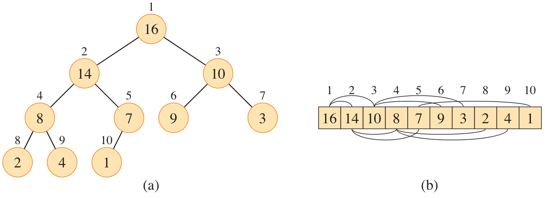
Get parents and children
Parent(i)
    return n//2

LeftChild(i)
    return n*2

RightChild(i)
    return n*2+1
We can use Bit operation:
Parent(i)
    return i >> 1        # i // 2

LeftChild(i)
    return i << 1        # i * 2

RightChild(i)
    return (i << 1) | 1  # i * 2 +1
Maintain a heap - $O(\log n)$
We have min-heap and max-heap, here, take max-heap as example,
MAX-HEAPIFY(A,i)
l = LEFT(i)
r = RIGHT(i)
if l <= A.heqp-size and A[l] > A[r]
    largest = l
else largest = i
if r <= A.heap-size and A[r] > A[largest]
    largest = r
if largest ≠ i
    exchange A[i] with A[largest]
    MAX-HEAPIFY(A, largest)
Build a heap - $O(n)$
BUILD-MAX-HEAP(A,n)
A.heap-size = n
for i = n//2 downto 1
    MAX-HEAPIFY (A, i)
Heapsort(A,n)
HeapSort(A, n)
BUILD-MAX-HEAP(A,n)
for i=n downto 2
    exchange A[1] with A[i]
    A.heapsize -= 1
    MAX-HEAPIFY (A, 1)
Priority Queues
you can take the value in the array as the level of priority. So there are 2 things that you need to do additionally:
- How to insert a number in to the heap
- How to change the number of some specific position
- How to pop out the maximum value (highest priority)
7 Quicksort
The worst case is $O(N^2)$, the average is $O(n\log n)$
QUICKSORT(A, p, r)
if p < r
q = PARTITION(A, p, r)
QUICKSORT(A, p, q - 1)
QUICKSORT(A, q + 1, r)
PARTITION(A, p, r)
x = A[r]
i = p - 1 # the location of pivot
for j = p to r - 1
if A[j] <= x
i = i + 1
exchange A[i] with A[j]
exchange A[i + 1] with A[r]
return i + 1 Performance
Bad PARTITION will cause the algorithm to be $O(n^2)$. In this case, each time we pick up the biggest or the samllest value so each partition will take $O(n)$, so $T(n) = T(n-1) + T(0) + \Theta(n)$
Good PARTITION can have $\Theta(n \lg n)$. It will split the array to 2 sub-array of equal length. so $T(n) = 2T(n/2) + \Theta(n)$
Actually, we only need a fixed partition to have $\Theta(n \lg n)$, even it is 9/10 (the depth of the tree is $\log_{10/9} n$).
In the real world, the bad PARTITION cannot always happen, the average case is $\Theta(n \lg n)$.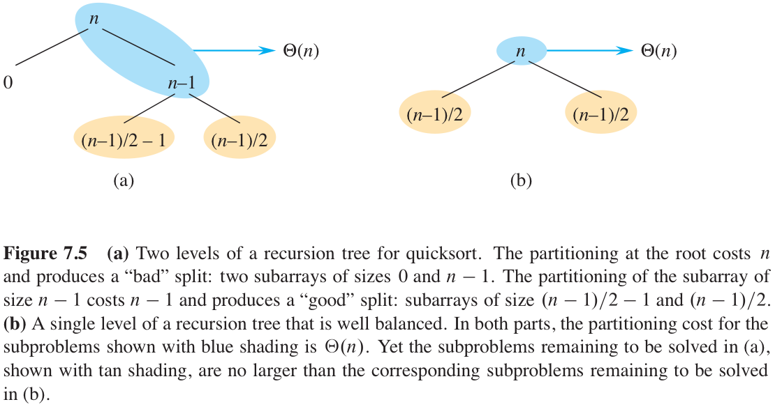
A randomized version of quicksort
RANDOMIZED-PARTITION(A, p, r)
    i = RANDOM(p, r)
    exchange A[r] with A[i]
    return PARTITION(A, p, r)
So now the running time is $\Theta(n \lg n)$
Some famous Problem
Hoare partition
HOARE-PARTITION(A, p, r)
x = A[p]                 // 1. 抓第一个人当基准典型
i = p - 1
j = r + 1
while TRUE
    repeat j = j - 1
        until A[j] <= x  // 右保镖:往左走,直到抓到 <= x 的人
    repeat i = i + 1
        until A[i] >= x  // 左保镖:往右走,直到抓到 >= x 的人
    if i < j
        exchange A[i] with A[j]  // 还没碰头?互相交换!
    else return j                // 碰头了?收工,返回刀口位置 j
Quicksort with equal element values
The PARTITION procedure returns an index q such that each element of A[p:q - 1] is less than or equal to A[q] and each element of A[q + 1:r]is greater than A[q].
Modify the PARTITION procedure to produce a procedure PARTITION(A,p,r),which permutes the elements of A[p:r] and returns two indices $q$ and $r$, where $p \le q \le t \le r$, such that
- all elements of A[q :t] are equal,
- each element of A[p:q - 1] is less than A[q], and
- each element of A[t + 1:r] is greater than A[g]
your PARTITION procedure should take O(r-p) time.
def PARTITION(A, p, r):
    pivot = A[r]

    lt = p
    gt = r

    j = p
    while j <= gt:
        if A[j] < pivot:
            A[lt], A[j] = A[j], A[lt]
            lt += 1
            j += 1
        elif A[j] > pivot:
            A[gt], A[j] = A[j], A[gt]
            gt -= 1
            j += 1
        else:
            j += 1
    return lt, gt
Alternative randomized versions
It is same when we first do a randomization on the array and run quickSort. In 7.3 we randomized in the partition. Mathmatically, it is the same. However, we don't use Alternative randomized versions in practics because of Cache Locality.
8 Counting sort - linear time
All the algorithm we discussed so far is comparison sort. Comparison sort can be thought as a decision tree, each time we compare 2 numbers and choose the bigger/smaller one.
To achieve linear time, we need Counting sort, Radix sort, Buket sort
Counting sort
Require the input array be an integer between 0 to k
COUNTING-SORT(A, B, k)
let B[1:n], C[0..k] be a new array
for i = 0 to k
    C[i] = 0

for j = 1 to A.length
    C[A[j]] = C[A[j]] + 1
// C[i] now contains the number of elements equal to i.

for i = 1 to k
    C[i] = C[i] + C[i - 1]
// C[i] now contains the number of elements less than or equal to i.

for j = A.length downto 1
    B[C[A[j]]] = A[j]
    C[A[j]] = C[A[j]] - 1
Time: $O(n+k)$, space $O(n+k)$
Radix Sort
Require the input number to have the same length
RADIX-SORT(A, d)
for i = 1 to d
    use a stable sort to sort array A on digit i
Time: $O(d(n+k))$Stable sort (Merge Sort, Counting Sort, Radix Sort, Insertion Sort). Heap Sort and Quicksort is not stable.
Bucket Sort
Require the input is drawn form a uniform distribution.
【original A】
[0.78, 0.17, 0.39, 0.26, 0.72, 0.94, 0.21, 0.12, 0.23, 0.68]

【Bcket B】
[0] -> /
[1] -> [0.12] -> [0.17]
[4] -> [0.21] -> [0.23] -> [0.26]
[5] -> [0.39]
[6] -> /
[5] -> /
[6] -> [0.68]
[7] -> [0.72] -> [0.78]
[8] -> /
[9] -> [0.94]

【output】
[0.12, 0.17, 0.21, 0.23, 0.26, 0.39, 0.68, 0.72, 0.78, 0.94]
A [1:n]
BUCKET-SORT(A)
let B[0..n-1] be a new array
n = A.length
for i = 0 to n - 1
make B[i] an empty list
for i = 1 to n
insert A[i] into list B[⌊n * A[i]⌋]
for i = 0 to n - 1
sort list B[i] with insertion sort
concatenate the lists B[0], B[1], ..., B[n-1] together in orderInsertion sort is $O(n^2)$, why Bucket Sort is $O(n)$? because if all the number is uniformly distributed, the expected time to sort the elements in each bucket using insertion sort is $O(1)$. Therefore, the total expected running time of bucket sort is $O(n)$.
some probelms
Sorting variable-length items
Sort items by their lengths first using counting sort, then apply radix sort from the most significant characters backwards to avoid scanning empty padding.
Water jugs
We have blue jugs and red jugs with various sizes, but you can only compare the capacity of a red jug with a blue jug. how to sort them in O(nlogn)?
This is a randomized quicksort variant. Use a red jug as a pivot to partition the blue jugs, and then use the matching blue jug to partition the red jugs.
k-sort
A $k$-sorted array can be decomposed into $k$ interwoven fully sorted subarrays. Sorting it completely takes $O(n \lg(n/k))$ time.
Lower bound on merging sorted lists
The information-theoretic lower bound for merging two sorted lists of sizes $n$ and $m$ is exactly $\lceil \lg \binom{n+m}{n} \rceil (C^n_{n+m})$. $C^n_{n+m}$ is the time you need to compare betwee 2 sorted arraies.
The 0-1 sorting lemma
The 0-1 Sorting Lemma states that if a comparison-based sorting network can correctly sort all possible inputs of 0s and 1s, it can correctly sort any input of arbitrary numbers.
9 Medians and Order Statistics
The $i$ th order statistic of a set of $n$ elements is the $i$ th smallest element. For example,
- the minimum of a set of elements is the first order statistic ($i = 1$), and
- the maximum is the $n$ th order statistic ($i = n$).
A median, informally, is the "halfway point" of the set.
- When n is odd, the median is unique, occurring at $\lfloor(n+1)/2\rfloor$.
- When n is even, there are two medians, the lower median occurring at $n/2$ and the upper median occurring at $n/2 + 1$ .
For simplicity in this text, however, we consistently use the phrase the median to refer to the lower median.
Selection Problem
MIN and MAX
Finding either takes exactly $n-1$ comparisons in the worst case. Instead of processing elements independently (taking $2n-2$ comparisons), we can process elements in pairs. By comparing elements of a pair with each other first, and then with the current min and max, the total number of comparisons is reduced to at most $3\lfloor n/2 \rfloor$.
Randomized-Select
Randomized-Select finds the $i$-th smallest element by modifying randomized quicksort.
It partitions the array around a random pivot. Unlike quicksort which recursively sorts both sides, Randomized-Select only recurses into one side that contains the target element, discarding the other side.
Under a uniform random strategy, the expected size of the remaining array drops geometrically ($n \rightarrow n/2 \rightarrow n/4 \dots$). The total cost is $n + n/2 + n/4 + \dots \le 2n = O(n)$ (linear time).
Worst-Case Time: If partitioning is completely unbalanced (e.g., pulling the max/min every time), the runtime degrades to $O(n^2)$.
BFPRT Algorithm
To avoid the worst case, we spent a little time to secure a perfect median
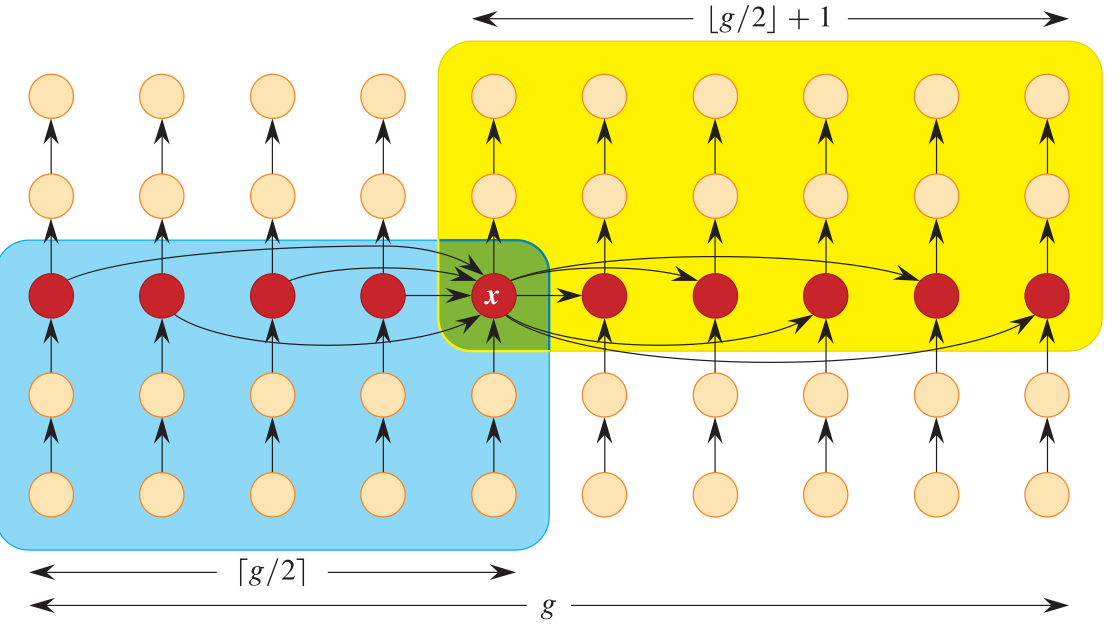
- Divide the $n$ elements into groups of $5$.
- Find the median of each group by insertion sort.
- Recursively find the median of these $\lceil n/5 \rceil$ medians, called $x$.
- Partition the entire array around $x$.
- Recurse into one side if the rank doesn't match.
$$T(n) \le T(n/5) + T(7n/10) + O(n)$$
T(n/5) is insertion sort cost, 7/10 is that for the value less then pivot
Summary of chapter 1-9
| Algorithm Name | Core Strategy | Best Time | Worst Time | Average Time | Space Complexity | Stable? |
|---|---|---|---|---|---|---|
| Insertion Sort | The Card-Shuffling Method. Keep a sorted hand of cards. Pick a new card and scan backward until you find its correct position to insert. | $O(n)$ (Already sorted) | $O(n^2)$ (Reversed input) | $O(n^2)$ | $O(1)$ (In-place) | Yes ✓ |
| Merge Sort | Divide and Conquer. Split the array cleanly down the middle, sort each half independently, and merge them back together using a temporary workspace. | $O(n \lg n)$ | $O(n \lg n)$ | $O(n \lg n)$ | $O(n)$ (Requires auxiliary space) | Yes ✓ |
| Heap Sort | The Tournament Tree. Build a Max-Heap. Repeatedly swap the root (maximum element) with the last element, remove it from the heap, and run Max-Heapify. | $O(n \lg n)$ | $O(n \lg n)$ | $O(n \lg n)$ | $O(1)$ (In-place) | No ✗ (Long-distance swaps) |
| Quicksort | Pivot Partitioning. Select a pivot element. Shuffle smaller values to the left and larger values to the right. Recursively repeat on both sides. | $O(n \lg n)$ | $O(n^2)$ (Extremely skewed pivot) | $O(n \lg n)$ | $O(\lg n)$ (Call stack overhead) | No ✗ |
| Counting Sort | Direct Indexing. Non-comparative. Count the frequencies of each value, compute their absolute starting positions, and place them directly into the output array. | $O(n + k)$ | $O(n + k)$ | $O(n + k)$ | $O(n + k)$ (Auxiliary array & counts) | Yes ✓ |
| Radix Sort | Digit-by-Digit Sorting. Sort the array least-significant digit to most-significant digit using a stable sort (like Counting Sort) as the underlying engine. | $O(d(n + k))$ | $O(d(n + k))$ | $O(d(n + k))$ | $O(n + k)$ | Yes ✓ (Requires stable base sort) |
| Bucket Sort | Interval Distribution. Divide the interval $[0, 1)$ uniformly into $n$ buckets. Distribute elements into buckets, sort each bucket using Insertion Sort, and concatenate. | $O(n)$ (Uniform distribution) | $O(n^2)$ (All items in one bucket) | $O(n)$ | $O(n)$ | Yes ✓ |
| Minimum / Maximum | Linear Scanning. Set the first element as the current champion, then compare it sequentially against the remaining $n-1$ elements. | $O(n)$ (Exactly $n-1$ comparisons) | $O(n)$ | $O(n)$ | $O(1)$ | — |
| Simultaneous Min-Max | Pairwise Dueling. Do not scan separately. Process elements in pairs first. Compare the winner to the global max and the loser to the global min. Saves 25% of comparisons. | $O(n)$ (Exactly $3\lfloor n/2 \rfloor$ comparisons) | $O(n)$ | $O(n)$ | $O(1)$ | — |
| Randomized Select | One-Sided Quick-Selection. Run Quicksort partitioning. Prune the search space by immediately discarding the partition that cannot contain the target index. | $O(n)$ | $O(n^2)$ (Worst-case partitions) | $O(n)$ | $O(\lg n)$ (Recursive, can be optimized to $O(1)$) | — |