Chapter 10-13 - Data structure

Reading material: book
Chapter 10-13

Some basic Algorithms: Chapter 1-9
We gonna to see

Array
Matrices
Stacks and Queues
Linked List
Binary trees
Hash Tables
Binary Search Trees
Red-Black trees

10 Elementary Data structure

Stack

LIFO

`PUSH` and `POP`

Time: $O(1)$.

STACK-EMPTY(S)
if S.top == 0
    return TRUE
else
    return FALSE

PUSH(S, x)
S.top = S.top + 1
S[S.top] = x

POP(S)
if STACK-EMPTY(S)
    error "underflow"
else
    S.top = S.top - 1
    return S[S.top + 1]

Queue

FIFO
Time: $O(1)$.

ENQUEUE(Q, x)
Q[Q.tail] = x
// reach the max and point to head
if Q.tail == Q.length
    Q.tail = 1
else
    Q.tail = Q.tail + 1

DEQUEUE(Q)
x = Q[Q.head]
if Q.head == Q.length
    Q.head = 1
else
    Q.head = Q.head + 1
return x

Linked list

not continous space

LIST-SEARCH takes $O(n)$ time.
LIST-INSERT and LIST-DELETE take $O(1)$ time (if the element node position is already known).

Singly Linked List

Doubly Linked List

Circular List

LIST-SEARCH(L, k)
x = L.head
while x != NIL and x.key != k
    x = x.next
return x

LIST-INSERT(L, x)
x.next = L.head
if L.head != NIL
    L.head.prev = x
L.head = x
x.prev = NIL

LIST-DELETE(L, x)
if x.prev != NIL
    x.prev.next = x.next
else
    L.head = x.next
if x.next != NIL
    x.next.prev = x.prev

Rooted trees

For binary tree, each node can have a left and right child. What if we have unbounded childen for a node?

Fortunately, there is a clever scheme to represent trees with arbitrary numbers of children. It has the advantage of using only $O(n)$ space for any n-node rooted tree.

As before, each node contains a parent pointer p, and T.root points to the root of tree T. Instead of having a pointer to each of its children, however, each node x has only two pointers:

x.left-child points to the leftmost child of node x , and
x.right-sibling points to the sibling of x immediately to its right.

alt text

11 hash table

Direct-address tables

Direct addressing is a simple technique that works well when the universe U of keys is reasonably small. Suppose that an application needs a dynamic set in which each element has a distinct key drawn from the universe $U = {0,1,...m-1}$, where m is not too large.

The dictionary operations DIRECT-ADDRESS-SEARCH, DIRECT-ADDRESS-INSERT, and DIRECT-ADDRESS-DELETE on the following page are trivial to implement. Each takes only $O(1)$ time.

Hash table

With direct addressing, an element with key k is stored in slot k, but with hashing,we use a hash function to compute the slot number from the key k,so that the element goes into slot $h(k)$. The hash function h maps the universe of keys into the slots of a hash table $T[0 : m - 1]$:
$$h:U→{0.1....,m-1}$$

Independent uniform hashing

Definition: An idealized mathematical assumption where any given key $k$ is equally likely to hash into any of the $m$ slots in the hash table, completely independent of where any other key has hashed.The Probability: If the table has $m$ slots and currently holds $n$ keys, the probability that a new key hashes into a specific slot $j$ is exactly:$$P(h(k) = j) = \frac{1}{m}$$Load Factor ($\alpha$): The average number of elements stored in a single slot, defined as:$$\alpha = \frac{n}{m}$$The Reality Check: This is a purely theoretical assumption used to analyze average-case performance. In practice, achieving perfect independence is difficult, which is why we approximate it using robust functions like Double Hashing or Universal Hashing.

Collision resolution by chaining

Core Strategy: Instead of searching for an open spot in the main array when a collision occurs, each slot $T[j]$ in the hash table points to a linked list (or basket) of all elements that hash to index $j$.List Selection: Using a doubly linked list is preferred because it allows for $O(1)$ time deletion when a pointer to the target node is provided.

Worst-case Search $O(n)$, everyone in the same bucket
Average-case, $O(1+n/m)$

Hash Function

A good Hash Function should satisfies: each key is equally likely to hash to any of the m slots, independently of where any other keys have hashed to. Unfortunately, you typically have no way to check this condition, unless you happen to know the probability distribution from which the keys are drawn.

In practice, a hash function is designed to handle keys that are one of the following two types:

A short nonnegative integer that fits in a w-bit machine word. Typical values for w would be 32 or 64.
A short vector of nonnegative integers, each of bounded size. For example, each element might be an 8-bit byte, in which case the vector is often called a (byte) string. The vector might be of variable length.

Static Hashing

The division method

$$h(k) = k \bmod m$$
Avoid choosing $m = 2^p$. Best to choose $m$ as a prime number not close to any power of 2.

The multiplication method

First, multiply the key $k$ by a constant $A$ in the range $0 < A < 1$ and extract the fractional part of $kA$.
$$h(k) = \lfloor m (k A \bmod 1) \rfloor$$

Works well with $m = 2^r$. Optimal choice for constant $A$ is the Golden Ratio $(\sqrt{5}-1)/2 \approx 0.6180339887$.

The multiply-based method
because floating-point arithmetic is slow.
$$s = \lfloor A \cdot 2^w \rfloor$$
$$h(k) = (k \cdot s) \bmod 2^w \gg (w - r)$$

Randm hashing (Universal hashing)

Using universal hashing and collision resolution by chaining in an initially empty table with $n$ slots, it takes $O(s)$ expected time to handle any sequence of $s$ INSERT, SEARCH,and DELETE operations containing $n = O(m)$ INSERT operations.

The INSERT and DELETE operations take constant time

INSERT: Under collision resolution by chaining, inserting a new element $x$ is done by simply splicing it into the head of the doubly linked list at slot $T[h(x.\text{key})]$. This always takes $O(1)$ worst-case time.

DELETE: Under the assumption that the operation is passed a pointer to the node to be deleted in a doubly linked list, updating the neighboring pointers takes $O(1)$ worst-case time.

Load Factor Boundary
The total number of keys inserted into the hash table throughout the sequence is $n$, and the total number of slots is $m$. By the theorem's premise, we have $n = O(m)$. The load factor $\alpha$ is defined as:$$\alpha = \frac{n}{m}$$Since $n = O(m)$, there exists a constant $c$ such that $n \le c \cdot m$. Therefore:$$\alpha = \frac{n}{m} \le c = O(1)$$The average number of keys per slot is bounded by a constant.

The Search is $O(1)$

Because of the load boundary is $\frac{n}{m}$

Using a universal family of hash functions here instead of using independent uniform hashing changes the probability of collision from 1/m to at most 1/m.
$$\Pr(h(k) = h(x)) \le \frac{1}{m}$$

Hashing long inputs such as vectors or strings

Polynomial Rolling Hash

$$h(X) = (x_0 \cdot a^r + x_1 \cdot a^{r-1} + \dots + x_{r-1} \cdot a^1 + x_r \cdot a^0) \bmod m$$

Horner's Rule

hash = 0
for each character x in X:
    hash = (hash * a + x) mod m

Open Addressing

Different from chaining, having a linked list on each seat. In Open Addressing, all elements are stored directly in the hash table itself.

The Probe Sequence

When a collision occurs, we systematically examine (or probe) other slots in the table until we find an empty one.
$$h(k, i)$$
where $k$ is the key, and $i$ is the probe number ($i = 0, 1, \dots, m-1$).

Linear Probing

$$h(k, i) = (h'(k) + i) \bmod m$$
If the initial slot is occupied, sequentially check the adjacent slots to the right: $h'(k)+1$, $h'(k)+2$, $h'(k)+3$, and so on.
As the table fills, long runs of contiguous occupied slots build up. If any slot in a cluster is hit, the entire cluster must be scanned, and the cluster grows even longer.

Quadratic Probing

$$h(k, i) = (h'(k) + c_1 i + c_2 i^2) \bmod m$$
Instead of step-by-step linear increments, the probe offsets grow quadratically (e.g., jumping by $1, 4, 9, 16, \dots$ slots).

While it avoids primary clustering, a milder form of clustering persists. If two keys share the same initial home slot (meaning $h'(k_1) = h'(k_2)$), they will traverse the exact same sequence of subsequent probes, resulting in collisions all the way down their paths.

Double Hashing (The Best Method)

$$h(k, i) = (h_1(k) + i \cdot h_2(k)) \bmod m$$
he first hash function $h_1(k)$ determines the initial starting slot, while the second hash function $h_2(k)$ determines the step-size (offset) for subsequent probes.

Min Insert time
Given an open-address hash table with load factor $\alpha = n/m < 1$ , the expected number of probes in an unsuccessful search is at most $$U(\alpha) \approx \frac{1}{1-\alpha}$$ assuming independent uniform permutation hashing and no deletions.

Max Search time
A search for a key $k$ reproduces the same probe sequence as when the element with key $k$ was inserted. If k was the $(i +1)st$ key inserted into the hash table, then the load factor at the time it was inserted was $i/m$, and so the expected number of probes made in a search for $k$ is at most $1/(1 - i/m) = m/(m-i)$. Averaging over all $n$ keys in the hash table gives us the expected number of probes in a successful search:
$$\frac{1}{n} \sum_{i=0}^{n-1} \frac{m}{m - i}$$
$$= \frac{m}{n} \sum_{i=0}^{n-1} \frac{1}{m - i}$$
$$= \frac{1}{\alpha} \sum_{i=0}^{n-1} \frac{1}{m - i}$$
From $\frac{1}{m-n+1}$ to $\frac{1}{m}$

$$\sum_{k=m-n+1}^{m} \frac{1}{k} \le \int_{m-n}^{m} \frac{1}{x} \, dx$$
$$\int_{m-n}^{m} \frac{1}{x} \, dx = [\ln(x)]_{m-n}^{m} = \ln(m) - \ln(m-n)= \ln\left(\frac{m}{m-n}\right) $$
$$S(\alpha) \le \frac{1}{\alpha} \ln \left( \frac{1}{1-\alpha} \right)$$

12 Binary Search Trees

We can express BST as a double linked list.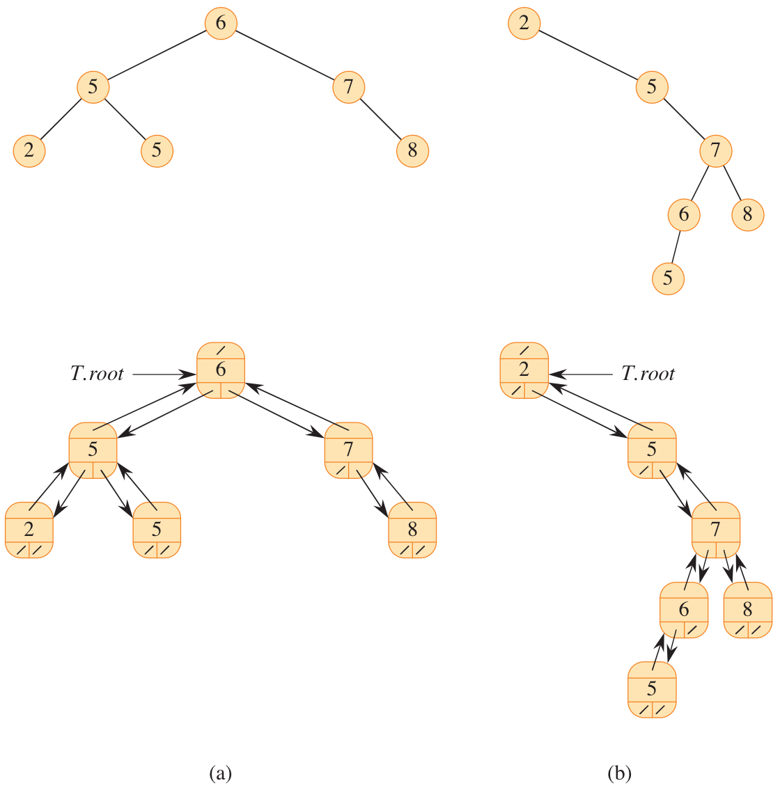

Inorder - Leetcode 94

left -> root -> right
if this is a sorted array, walk-inorder will produce a ascending results

Preorder

root -> left -> right

Postorder

right -> left -> root

All the walk takes $O(n)$

Search in a binary tree

related to the hight of tree $h$.

ITERATIVE-TREE-SEARCH(x, k)
while x != NIL and k != x.key
    if k < x.key
        x = x.left
    else
        x = x.right
return x

`MIN` and `MAX`

TREE-MINIMUM(x)
while x.left != NIL
    x = x.left
return x

SUCCESSOR(x)

Case A: Node $x$ has a non-empty right subtree ($x.\text{right} \ne \text{NIL}$)Mechanism: The successor is the smallest element in $x$'s right subtree.Rule: Go to the right child, and then find the minimum of that subtree.Computation:$$\text{Successor}(x) = \text{TREE-MINIMUM}(x.\text{right})$$

Case B: Node $x$ has an empty right subtree ($x.\text{right} = \text{NIL}$)Mechanism: We must go up the tree to search among $x$'s ancestors. We ascend the parent pointers until we find an ancestor node $y$ such that $x$ falls into $y$'s left subtree.Rule: Follow parent pointers up until we make our first right turn (i.e., we are no longer a right child of our parent).

TREE-SUCCESSOR(x)
if x.right != NIL
    return TREE-MINIMUM(x.right)
y = x.p
while y != NIL and x == y.right
    x = y
    y = y.p
return y

Insertion and Deletion

Insertion

Insertion Time Complexity: $O(h)$, where $h$ is the height of the tree.

TREE-INSERT(T, z)
y = NIL
x = T.root
while x != NIL                      // Traverse to find the parent 'y'
    y = x
    if z.key < x.key
        x = x.left
    else
        x = x.right
z.p = y                             // Set z's parent to y
if y == NIL
    T.root = z                      // Tree was empty
elif z.key < y.key
    y.left = z
else
    y.right = z

Deletion

// use v to replace u

TRANSPLANT(T, u, v)
if u.p == NIL
    T.root = v

// is left child
elif u == u.p.left
    u.p.left = v
else
    u.p.right = v

if v != NIL
    v.p = u.p

The Three Cases of Deletion:

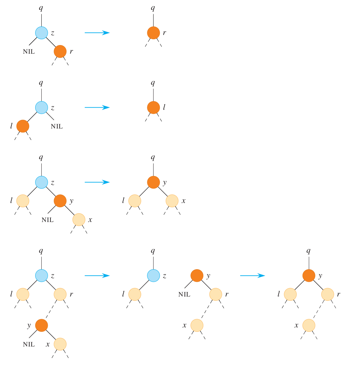
Case 1: No Children (Leaf Node)Mechanism: Node $z$ is a leaf. We simply disconnect it from its parent by calling TRANSPLANT(T, z, NIL).
Case 2: One Child (Single Descendant)Mechanism: Node $z$ has only one child $v$ (either left or right). We promote $v$ to take $z$'s place in the tree, connecting $v$ directly to $z$'s parent.Execution: TRANSPLANT(T, z, z.left) or TRANSPLANT(T, z, z.right).
Case 3: Two Children (Symmetric Successor Replacement)Mechanism: Node $z$ has both a left and a right child. We cannot simply delete it. Instead, we must find $z$'s successor $y$ (which lies in $z$'s right subtree and has no left child), move $y$ to $z$'s position, and re-link $z$'s original left and right subtrees to $y$.
- Subcase 3a (y is z's right child):We replace $z$ with $y$ using TRANSPLANT(T, z, y) and set $y.\text{left} = z.\text{left}$.
- Subcase 3b (y lies deeper in z's right subtree):Replace $y$ with its own right child $y.\text{right}$ via TRANSPLANT(T, y, y.right). Set $y.\text{right} = z.\text{right}$ and update parent pointers.Replace $z$ with $y$ via TRANSPLANT(T, z, y) and set $y.\text{left} = z.\text{left}$.

> case b->case a, than do case a

如果大堂经理运气不好，按 1, 2, 3, 4, 5 的升序顺序把人插入树中：这棵树就会长成一个往右边一路斜向下的“拐杖”（单链表）！此时树的高度 $h = n$。所有操作的辛苦费全从完美的 $O(\lg n)$ 暴跌回 $O(n)$！为了不让 BST 变成一根拐杖，红黑树正式登场！

13 Red-black Trees

Every node is either red or black.
The root is black.
Every leaf (NIL) is black.
If a node is red, then both its children are black.
For each node, all simple paths from the node to descendant leaves contain the same number of black nodes.

when the red-black tree satisfies the 5 rules, we can see the max height of this tree is $2 \lg(n+1)$. Therefore, Search, Insert, Delete are all $O(\lg n)$！

Rotation - O(1)

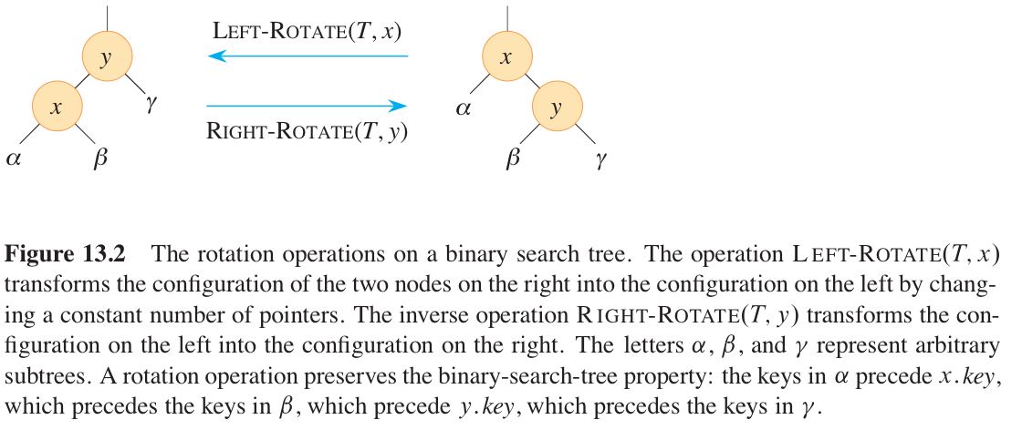
LEFT-ROTATE(T, x)
y = x.right                     // Set y to be x's right child
x.right = y.left                // Turn y's left subtree into x's right subtree

if y.left != T.nil              // If y's left subtree is not empty...
    y.left.p = x                // ...then x becomes the parent of that subtree's root

y.p = x.p                       // Link x's parent to y

if x.p == T.nil                 // If x was the root of the entire tree...
    T.root = y                  // ...then y becomes the new root
elif x == x.p.left              // Otherwise, if x was a left child...
    x.p.left = y                // ...then y becomes the new left child
else                            // Otherwise, x was a right child...
    x.p.right = y               // ...and now y becomes the new right child

y.left = x                      // Put x on y's left
x.p = y                         // Set y as x's parent

Insertion

When inserting a new node $z$, we perform standard TREE-INSERT(T, z) and initially color $z$ RED. Just like what we do in the BST, but color it red.

Why RED? Coloring $z$ red preserves Property 5 (black-height), but it might violate Property 4 (if $z$'s parent is also red).

RB-INSERT(T, z)
current = T.root                      // Node being compared with z
parent = T.nil                        // the parent of z
while current != T.nil                // Descend until reaching the sentinel
    parent = current
    if z.key < current.key
        current = current.left
    else
        current = current.right
z.p = parent                         // Found the location to insert z with parent y
if parent == T.nil
    T.root = z                  // Tree T was empty
elif z.key < parent.key
    parent.left = z
else
    parent.right = z

z.left = T.nil                  // Both of z's children are the sentinel (T.nil)
z.right = T.nil
z.color = RED                   // The new node starts out RED

RB-INSERT-FIXUP(T, z)           // Correct any violations of red-black properties

To fix any red-red violations, we call RB-INSERT-FIXUP(T, z).

RB-INSERT-FIXUP(T, z)
while z.p.color == RED
    if z.p == z.p.p.left        // Is z's parent a left child?
        y = z.p.p.right         // y is z's uncle
        
        if y.color == RED       // Case 1: Parent and uncle are both RED
            z.p.color = BLACK
            y.color = BLACK
            z.p.p.color = RED
            z = z.p.p           // Move z up to grandparent and repeat
        else 
            if z == z.p.right   // Case 2: Uncle is BLACK, and z is a right child
                z = z.p
                LEFT-ROTATE(T, z)
            
            // Case 3: Uncle is BLACK, and z is a left child
            z.p.color = BLACK
            z.p.p.color = RED
            RIGHT-ROTATE(T, z.p.p)
            
    else                        // Same as above, but with "right" and "left" exchanged
        y = z.p.p.left          // y is z's uncle
        
        if y.color == RED       // Case 1 (Symmetric)
            z.p.color = BLACK
            y.color = BLACK
            z.p.p.color = RED
            z = z.p.p
        else
            if z == z.p.left    // Case 2 (Symmetric)
                z = z.p
                RIGHT-ROTATE(T, z)
            
            // Case 3 (Symmetric)
            z.p.color = BLACK
            z.p.p.color = RED
            LEFT-ROTATE(T, z.p.p)

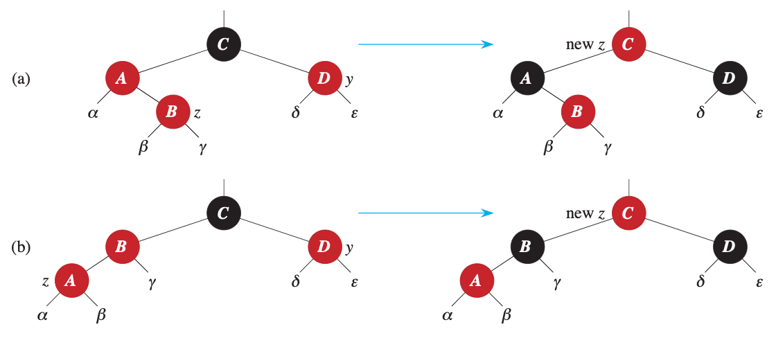
T.root.color = BLACK            // Ensure the root is always BLACK (Property 2)

Case 1: $z$'s uncle $y$ is RED:
Both parent $z.p$ and uncle $y$ are red.Action (Recolor):Color parent $z.p$ and uncle $y$ BLACK. Color grandparent $z.p.p$ RED.Move the pointer $z \leftarrow z.p.p$ up to the grandparent and repeat.

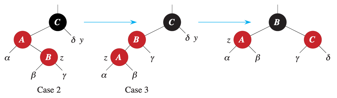
Case 2: $z$'s uncle $y$ is BLACK and $z$ is a "Right Child" (Zig-Zag Shape)
Condition: Uncle $y$ is black, and $z$ forms a triangle/bend with parent and grandparent.Action (Rotate to straighten): Set $z \leftarrow z.p$. Call LEFT-ROTATE(T, z) to transform Case 2 into Case 3 (straight line).

Case 3: $z$'s uncle $y$ is BLACK and $z$ is a "Left Child" (Straight Line Shape):
Uncle $y$ is black, and $z$ is collinear with parent and grandparent.Action (Recolor and Rotate): Color parent $z.p$ BLACK.Color grandparent $z.p.p$ RED.Call RIGHT-ROTATE(T, z.p.p). The loop terminates because $z$'s parent is now black (Property 4 is restored).

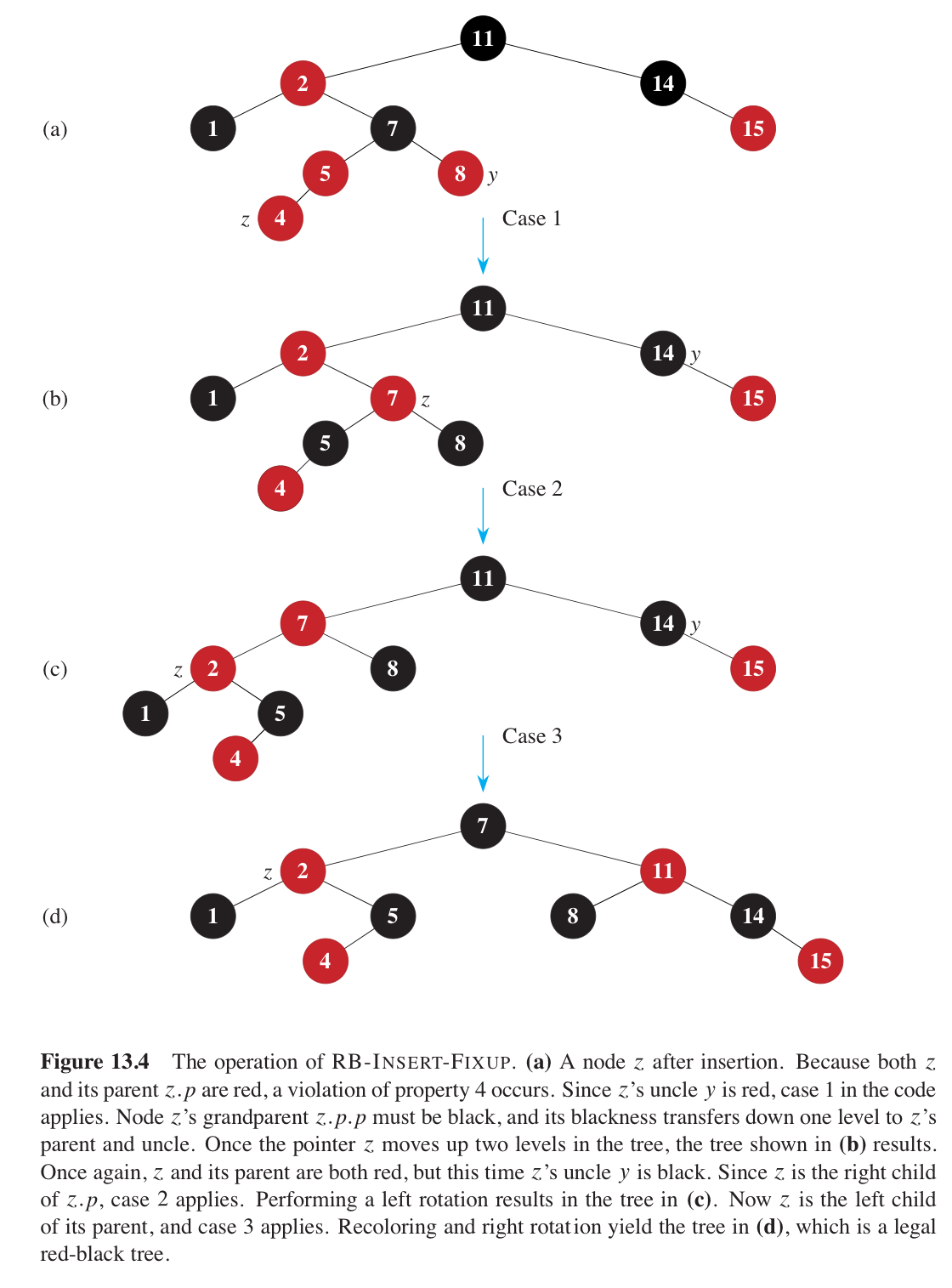
Whole Example:

Deletion

If we delete a red node, everything will be ok, we don't need a fixup.

But if we delete a black node, we need to fix up to solve the conflicts.

RB-DELETE(T, z)
y = z
y-original-color = y.color
if z.left == T.nil
    x = z.right
    RB-TRANSPLANT(T, z, z.right)            // replace z by its right child
elseif z.right == T.nil
    x = z.left
    RB-TRANSPLANT(T, z, z.left)             // replace z by its left child
else y = TREE-MINIMUM(z.right)               // y is z's successor
    y-original-color = y.color
    x = y.right
    if y != z.right                         // is y farther down the tree?
        RB-TRANSPLANT(T, y, y.right)        // replace y by its right child
        y.right = z.right                   // z's right child becomes
        y.right.p = y                       //     y's right child
    else x.p = y                            // in case x is T.nil
    RB-TRANSPLANT(T, z, y)                  // replace z by its successor y
    y.left = z.left                         // and give z's left child to y,
    y.left.p = y                            //     which had no left child
    y.color = z.color
if y-original-color == BLACK                // if any red-black violations occurred,
    RB-DELETE-FIXUP(T, x)                   //     correct them

So we should know why we do the fixup here. Because we deleted a black node, the tree is not balanced any more. So we should whatever add a black node or others to fix it.

for the node x, x is right child of the deleted node. If x is red, turn x to be black is enough. but if the x is already black, but we need to add one more black (Double-black).

Therefore, we want to find a red one and turn it into black, the only hope is to find a red child of x's brother. So that we can let that child to be black (obey red parent and black children), and rotate the black brother to x's side to add one more black on the path.

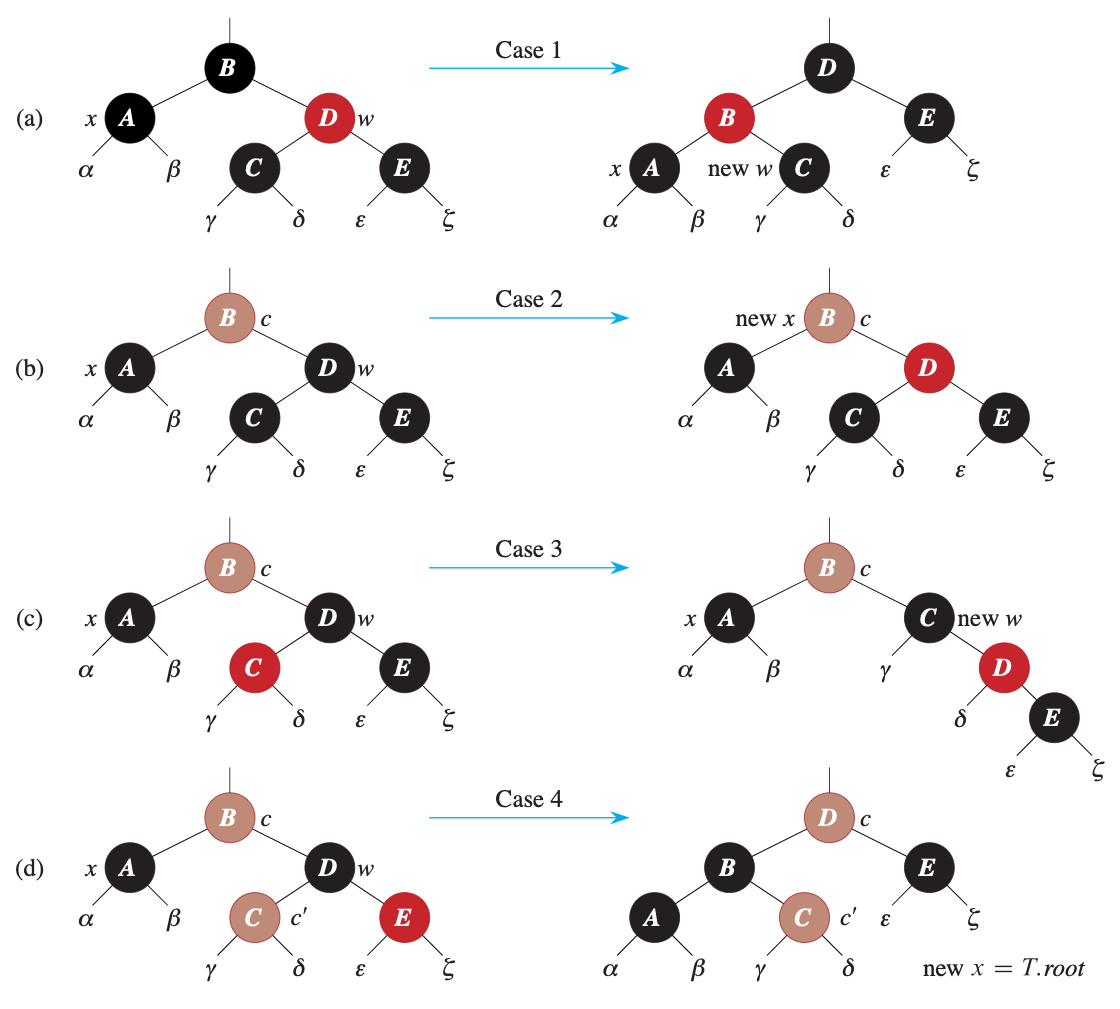
Case 1 brother is red, which means that his children is all black. turn this red brother into black and left rotate.
Case 2 brother is black, but have 2 black children, so turn it to be red, so brother now need a black as well, and let x be the father to find above
Case 3 brother is black, have a red right children, zig-zag to straight (case 4)
Case 4 brother is black, have a red left children, what we want

RB-DELETE-FIXUP(T, x)
while x != T.root and x.color == BLACK
    if x == x.p.left                        // is x a left child?
        w = x.p.right                       // w is x's sibling
        
        if w.color == RED
            w.color = BLACK                 // Case 1
            x.p.color = RED
            LEFT-ROTATE(T, x.p)
            w = x.p.right
            
        if w.left.color == BLACK and w.right.color == BLACK
            w.color = RED                   // Case 2
            x = x.p
        else
            if w.right.color == BLACK
                w.left.color = BLACK        // Case 3
                w.color = RED
                RIGHT-ROTATE(T, w)
                w = x.p.right
                
            w.color = x.p.color             // Case 4
            x.p.color = BLACK
            w.right.color = BLACK
            LEFT-ROTATE(T, x.p)
            x = T.root
            
    else                                    // same as above, but with "right" and "left" exchanged
        w = x.p.left
        
        if w.color == RED
            w.color = BLACK                 // Case 1 (Symmetric)
            x.p.color = RED
            RIGHT-ROTATE(T, x.p)
            w = x.p.left
            
        if w.right.color == BLACK and w.left.color == BLACK
            w.color = RED                   // Case 2 (Symmetric)
            x = x.p
        else
            if w.left.color == BLACK
                w.right.color = BLACK       // Case 3 (Symmetric)
                w.color = RED
                LEFT-ROTATE(T, w)
                w = x.p.left
                
            w.color = x.p.color             // Case 4 (Symmetric)
            x.p.color = BLACK
            w.left.color = BLACK
            RIGHT-ROTATE(T, x.p)
            x = T.root

x.color = BLACK

2026-07-15T19:51:13.png

> cat Chapter 10-13 - Data structure.md

10 Elementary Data structure

Stack

PUSH and POP

Queue

Linked list

Singly Linked List

Doubly Linked List

Circular List

Rooted trees

11 hash table

Direct-address tables

Hash table

Independent uniform hashing

Collision resolution by chaining

Hash Function

Static Hashing

The division method

The multiplication method

Randm hashing (Universal hashing)

Hashing long inputs such as vectors or strings

Polynomial Rolling Hash

Open Addressing

The Probe Sequence

Linear Probing

Quadratic Probing

Double Hashing (The Best Method)

12 Binary Search Trees

Inorder - Leetcode 94

Preorder

Postorder

Search in a binary tree

MIN and MAX

SUCCESSOR(x)

Insertion and Deletion

Insertion

Deletion

13 Red-black Trees

Rotation - O(1)

Insertion

Deletion

`PUSH` and `POP`

`MIN` and `MAX`