Previous:
Chapter 1-9: algorithm
Chapter 10-13: data structure
This part is called Advanced Design and Analysis Techniques. In chapter, we have learnt master method and Probabilistic Analysis and Randomized Algorithms. Here, we gonna to talk more about analysis.
14 Dynamic Programming
A dynamic-programming algorithm solves each subsubproblem just once and then saves its answer in a table, thereby avoiding the work of recomputing the answer every time it solves each subproblem. Mostly for Optimization Problems.
To develop a dynamic-programming algorithm, follow a sequence of four steps:
- Characterize the structure of an optimal solution.
- Recursively deûne the value of an optimal solution.
- Compute the value of an optimal solution, typically in a bottom-up fashion.
- Construct an optimal solution from computed information
Rod-cutting problem
Given a rod of length $n$ inches and a table of prices $p_i$ for $i = 1, 2, ... n$, determine the maximum revenue $r_n$ obtainable by cutting up the rod and selling the pieces.
Considering this question step by step, the profit we can get is the max price we can get by cutting the rod once in current state plus the max price we can get in previous steps.
$$R_n = \max_{1 \le i \le n} (p_i + R_{n-i})$$
If we write it recursively, we have $n$ possibilities to cut the rod each step:
CUT-ROD(p, n)
    if n == 0
        return 0
    q = -infinity
    for i = 1 to n
        // this step cuts i
        q = max(q, p[i] + CUT-ROD(p, n - i))
    return q
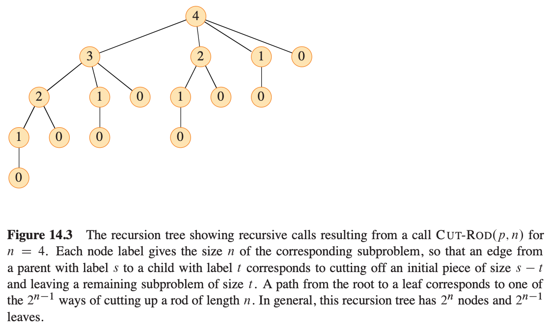
The execution tree grows exponentially because the algorithm repeatedly solves the exact same subproblems (e.g., calculating $T(1)$ and $T(2)$ over and over again).
Bottom-up
BOTTOM-UP-CUT-ROD(p, n)
    let r[0..n] be a new array       // r[j] 用来保存长度为 j 的钢条的最大收益
    r[0] = 0                         // 长度为 0 的钢条收益为 0

    for j = 1 to n                   // 外层循环:从小到大依次计算长度为 j 的钢条的最优解
        q = -infinity
        for i = 1 to j               // 内层循环:尝试在位置 i 切第一刀
            q = max(q, p[i] + r[j - i])  // 直接从我们已经算好的小账本 r 里查 r[j-i],O(1) 速度!
        r[j] = q                     // 把长度为 j 的最优解记入小账本

    return r[n]                      // 返回长度为 n 的最大收益
Top-Down with Memoization
MEMOIZED-CUT-ROD(p, n)
let r[0..n] be a new array       // will remember solution values in r
for i = 0 to n
    r[i] = -infinity
return MEMOIZED-CUT-ROD-AUX(p, n, r)

MEMOIZED-CUT-ROD-AUX(p, n, r)
if r[n] >= 0                     // already have a solution for length n?
    return r[n]
if n == 0
    q = 0
else q = -infinity
    for i = 1 to n               // i is the position of the first cut
        q = max(q, p[i] + MEMOIZED-CUT-ROD-AUX(p, n - i, r))
r[n] = q                         // remember the solution value for length n
return q
Matrix-chain multiplication
if we have 3 matrices $A_1 \times A_2 \times A_3$
- $A_1$: $10 \times 100$
- $A_2$: $100 \times 5$
- $A_3$: $5 \times 50$
if we do $((A_1 A_2) A_3)$
$10 \times 100 \times 5 + 10 \times 5 \times 50 = 7500 $
if we do $(A_1 (A_2 A_3))$
$100 \times 5 \times 50 + 10 \times 100 \times 50 = 75,000$
How to find an optimal combination?
If we use the divide-and-conquer, we will need $\Omega(2^n)$, DP can do it in $\Theta(n^3)$.
Assume we want to the multiply from $A_i$ to $A_j$, Let the minimum multiplication time from $A_i$ to $A_j$ is $m[i,j]$. For a $k (i \le k < j)$, $p$ is the size of matrix: The size of $A_i$ is $p_{i-1} \times p_i$
$$\text{p} = [p_0, p_1, p_2, \dots, p_n]$$
$$m[i, j] = \min_{i \le k < j} \Big( m[i, k] + m[k+1, j] + p_{i-1}p_k p_j \Big)$$
MATRIX-CHAIN-ORDER(p)
n = p.length - 1
let m[1..n, 1..n] and s[1..n-1, 2..n] be new tables

for i = 1 to n
    m[i, i] = 0                      // 长度为 1 的链(单个矩阵),不需要相乘,代价为 0

for l = 2 to n                       // l 是链的长度
    for i = 1 to n - l + 1
        j = i + l - 1
        m[i, j] = infinity
        for k = i to j - 1           // 尝试在 i 到 j-1 之间的每一个位置 k 劈开
            q = m[i, k] + m[k+1, j] + p[i-1] * p[k] * p[j]
            if q < m[i, j]
                m[i, j] = q          // 记下最省钱的乘法次数
                s[i, j] = k          // 记下最省钱的那一刀切在哪个位置

return m and s

PRINT-OPTIMAL-PARENS(s, i, j)
if i == j
    print "A" + i                     // 递归边界:只剩一个矩阵了,直接打印矩阵名字(如 A1)
else
    print "("                         // 要在 k 处劈开了,先打左括号
    PRINT-OPTIMAL-PARENS(s, i, s[i, j]) // 递归打印左半边:从 i 到 s[i, j]
    PRINT-OPTIMAL-PARENS(s, s[i, j] + 1, j) // 递归打印右半边:从 s[i, j] + 1 到 j
    print ")"                         // 两边都打完了,闭合右括号
Elements of DP
Optimal Substructure and Overlapping Subproblems.
Optimal Substructure
- Show that a solution to the problem consists of making a choice
- Assume that for a given problem, you are given the choice that leads to an optimal solution.
- Given this choice, determine which subproblems arise
- Prove that the solutions to the subproblems used within an optimal solution to the entire problem must themselves be optimal.
Optimal substructure fails if subproblems are not independent. Subproblem Independence means that solving one subproblem does not affect the resources available to solve another subproblem of the same optimal solution.Classic Example of Dependence (Longest Simple Path):
To find the longest simple path (a path with no repeated vertices) $s \to u \to t$, the subproblems $s \to u$ and $u \to t$ are dependent. If we find the longest simple path for $s \to u$, we may use up vertices that are required to make $u \to t$ as long as possible. Therefore, Longest Simple Path cannot be solved using Dynamic Programming.
Overlapping Subproblems
A recursive algorithm for the problem solves the same subproblems repeatedly, rather than generating new subproblems at each step.
In Divide-and-Conquer (like Merge Sort), the algorithm partitions the problem into brand-new, disjoint subproblems at each step.
Optimize DP
- Comparison Dimension 1: Constant-Factor Overhead (Winner: Bottom-Up)
When all subproblems in the subproblem space must be solved at least once (e.g., in Matrix-Chain Multiplication), the Bottom-Up approach is generally superior in practice. - Comparison Dimension 2: Subproblem Space Exploration (Winner: Memoization)
When only a subset of the subproblem space needs to be solved to compute the final optimal solution (a Sparse Subproblem Space), the Top-Down Memoized approach is far more efficient.
Longest common subsequence
Leetcode 1143 - here
For example, $Z = <B, C, D, B >$ is a subsequence of $Z = <A, B, C, B, D, A, B >$ with corresponding index sequence $<2, 3, 5, 7>$.
Let $X = \langle x_1, x_2, \dots, x_m \rangle$ and $Y = \langle y_1, y_2, \dots, y_n \rangle$ be two sequences. Let $Z = \langle z_1, z_2, \dots, z_k \rangle$ be any LCS of $X$ and $Y$.
- Case 1: $x_m = y_n$Then $z_k = x_m = y_n$, and $Z_{k-1}$ is an LCS of $X_{m-1}$ and $Y_{n-1}$.
- Case 2: $x_m \neq y_n$If $z_k \neq x_m$, then $Z$ is an LCS of $X_{m-1}$ and $Y$. If $z_k \neq y_n$, then $Z$ is an LCS of $X$ and $Y_{n-1}$.
Let $c[i, j]$ be the length of an LCS of prefixes $X_i$ and $Y_j$.
$$c[i, j] = \begin{cases} 0 & \text{if } i = 0 \text{ or } j = 0 \\ c[i-1, j-1] + 1 & \text{if } i, j > 0 \text{ and } x_i = y_j \\ \max(c[i-1, j], c[i, j-1]) & \text{if } i, j > 0 \text{ and } x_i \neq y_j \end{cases}$$
Time Complexity: $\Theta(mn)$ using bottom-up tabulation.
Optimal Binary Search tree
Given a sequence $K = \langle k_1, k_2, \dots, k_n \rangle$ of $n$ distinct keys in sorted order, and a set of $n+1$ dummy keys $D = \langle d_0, d_1, \dots, d_n \rangle$ representing searches that fall between keys.Each key $k_i$ has a search probability $p_i$. Each dummy key $d_i$ has a search probability $q_i$.The total probability is $\sum_{i=1}^n p_i + \sum_{i=0}^n q_i = 1$. We wish to construct a binary search tree that minimizes the expected search cost:$$\text{E}[\text{Search Cost}] = \sum_{i=1}^n (\text{depth}(k_i) + 1) \cdot p_i + \sum_{i=0}^n (\text{depth}(d_i) + 1) \cdot q_i$$
15 Greedy Algorithms
Algorithms for optimization problems typically go through a sequence of steps, with a set of choices at each step. For many optimization problems, using dynamic programming to determine the best choices is overkill, and simpler, more efficient algorithms will do. A greedy algorithm always makes the choice that looks best at the moment.
An activity-selection problem
You are presented with a set $S = {a_1, a_2, a_3,..., a_n}$ of $n$ proposed activities that wish to reserve the conference room, and the room can serve only one activity at a time. Select as much as possible activities!
If we use DP, so we assume we pick event $a_k$, we have to subquestion the max event before ad after $a_k$, so
$$e[i, j] = \max (e[i, k] + e[k, j] + 1)$$
It takes $O(n^3)$
However, if we are greedy enough, we always chose the event ends earliest and doesn't conflict with others.
- We pick $a_1$
- $a_4$ is the next ends earliest and don't conflicts
- $a_8$
- $a_{11}$
we only take $O(n)$ to solve this
RECURSIVE-ACTIVITY-SELECTOR(s, f, k, n)
  m = k + 1
  while m <= n and s[m] < f[k]    // 寻找在 Sk 中第一个与 ak 兼容(即开始时间 >= fk)的活动
      m = m + 1
  if m <= n
      return {a_m} ∪ RECURSIVE-ACTIVITY-SELECTOR(s, f, m, n)
  else
      return ∅
GREEDY-ACTIVITY-SELECTOR(s, f)
n = s.length
A = {a_1} // 贪心选择:第一个活动必选(因为它结束最早)
k = 1 // k 记录最近一次加入账本的活动
for m = 2 to n
if s[m] >= f[k] // 如果当前活动的开始时间不冲突
A = A ∪ {a_m} // 贪心地把它塞进日程表
k = m // 更新最近一次账目
return AElements of the greedy strategy
Greedy-choice property
A global optimal solution can be reached by making a locally optimal (greedy) choice. Make the best choice right now without worrying about the future.
Optimal substructure
Once you make your greedy choice, the remaining problem is just a smaller version of the original. If you solve the remaining part optimally, you get the overall optimal solution.
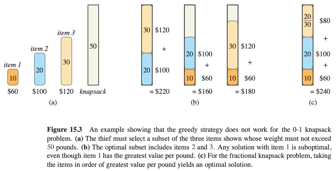
we cannot use greedy to solve 0-1 knapsack problem.
Huffman codes
Greedy strategy: Merges the two least frequent nodes at each step to build a tree from the bottom up.
Result: Highly frequent characters get shorter codes (near root); rare characters get longer codes (deep in tree), minimizing total file size.
Offline caching(Belady's Greedy Algorithm)
Greedy strategy: When the cache is full, evict the item whose next access is furthest in the future.
Result: Maximizes cache hits by exploiting complete future knowledge of the request sequence.
16 Amortized Analysis
Amortized analysis is stronger than average-case analysis. If an algorithm is $O(1)$ in average or expected time, it could be much worse, even the very first time we use it, just with low probability.
If something has $O(1)$ amortized time, that means you can do a sequence of $n$ operations, and the total running time of operations 1 to k never exceeds $O(k)$ even though an individual operation might exceed O(1).
Aggregate analysis is a form of amortized analysis. We know that adding the k'th point in the fast convex hull algorithm might take more than $O(1)$ if the while-loop iterates multiple times, even as much as $O(k)$, but the total cost of adding points 1 to k cannot exceed $O(k)$ because all the while-loops cannot remove more points than have been added.
For the persistent red-black tree, we need a stronger technique: save money in each node to pay for future operations.
Remember that we store in each node all the changes we make to its left and right pointers, but when the number of changes exceeds a constant, we replace the node (and change the left or right pointer of its parent).
Let's suppose we charge 2 to change the left or right pointer of a node. 1 pays for the operation, including allocating a new node if necessary, but not for changing the parent's pointer. The other $1, we store in the node. Suppose we allow at least two changes before reallocating a node.
That means that if we need to reallocate and therefore change the parent's left or right pointer, we will have 2 saved up to do it, which is exactly what we need.
The parent might have to be replaced, too, but then it will have 2 to pay for the grandparent. We never run out of money. However, we might end up spending $\log n$ of our saved money, meaning the actual (space) cost of an operation might be $O(\log k)$ even if the total never exceeds $O(k)$.
Since the system works if we charge 2 per change, 1 for the current change, and 1 for a future one, the number of extra changes never exceeds the number of red-black algorithm changes, so the total cost for $k$ operations is still a constant times $k$, and the amount of space used for storing all the trees is $O(n)$.
By the way, don't forget we are just trying to bound the amount of space used. n operations on a red-black tree costs $O(n log n)$ because of the lookups and color changes. However, it requires only a constant number of rotations per operation, and so a total of $O(n)$ left or right pointer changes.